Denoising and Detoning

This chapter explains why empirical covariance matrices are "noisy" and "ill-conditioned" and presents a method based on Random Matrix Theory (RMT) to clean them. Using a noisy matrix for portfolio optimization or risk analysis leads to unstable and poor results. This method separates the matrix into "signal" (true structure) and "noise" (randomness) to create a more robust matrix.

The Marcenko-Pastur Theorem

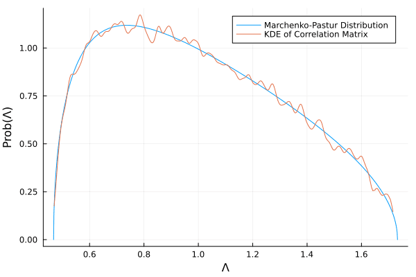
This is the theoretical foundation for separating signal from noise. It describes the Probability Density Function (PDF) of eigenvalues for a purely random covariance matrix $C$ of size $T \times N$.

• Key Insight: Any eigenvalues from an empirical matrix that fall inside the Marcenko-Pastur distribution are considered noise. Any eigenvalues that fall outside (specifically, larger than $\lambda_+$) are considered signal.
• The theory provides a clear-cut maximum eigenvalue $\lambda_+$ for a random matrix:
  $$\lambda_{+} = \sigma^{2}(1+\sqrt{N / T})^{2}$$
• The full PDF is given by:
  $$f[\lambda]= \frac{T}{N} \frac{\sqrt{\left(\lambda_{+}-\lambda\right)\left(\lambda-\lambda_{-}\right)}}{2 \pi \lambda \sigma^{2}}$$

To apply this, the algorithm fits this theoretical PDF to the empirical distribution of eigenvalues to find the data-driven cutoff $\lambda_+$ that best separates random components from structural components.

Denoising

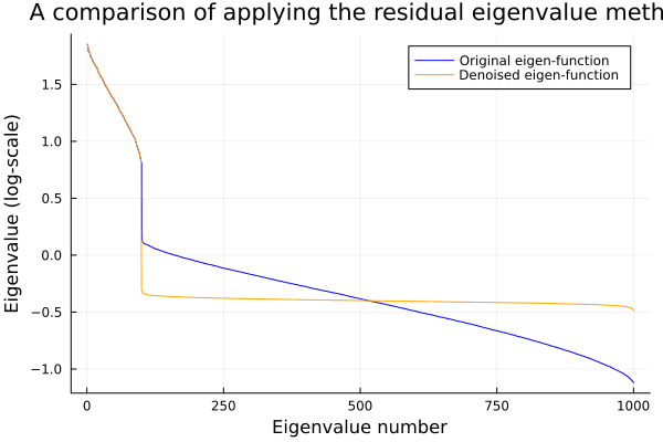
Denoising is the process of removing the noise identified by the Marcenko-Pastur theorem, while preserving the signal. This is superior to standard "shrinkage" (like Ledoit-Wolf), which dilutes both signal and noise.

The primary method described is the Constant Residual Eigenvalue Method:

1. Identify all noise eigenvalues ($\lambda_n \le \lambda_+$) and all signal eigenvalues ($\lambda_n > \lambda_+$).
2. Replace all noise eigenvalues with their average: $\lambda_{j}= \frac{1}{(N-i)} \sum_{k=i+1}^{N} \lambda_{k}$.
3. The signal eigenvalues are left untouched.
4. The new, "clean" correlation matrix $\widetilde{C}_1$ is re-built using the original eigenvectors ($W$) and the modified eigenvalues ($\widetilde{\Lambda}$).
   $$\widetilde{C}_{1} = W \widetilde{\Lambda} W^{\prime}$$

(The matrix is then rescaled to have 1s on the diagonal, creating $C_1$).

Detoning

Detoning is the process of removing the dominant market-wide component (the "tone") from the denoised matrix $C_1$. This is useful for clustering and finding more subtle, non-market-related structures (like sectors).

1. The market component is identified (usually the first eigenvector, $W_M$).
2. This component is explicitly subtracted from the denoised matrix:
   $$\widetilde{C}_{2} = C_{1} - W_{M} \Lambda_{M} W_{M}^{\prime}$$
3. The resulting "detoned" matrix $C_2$ is singular (not invertible) but is now much better for identifying clusters. For optimization, one can optimize on the remaining principal components ($f^*$) and map the weights back to the original assets:
   $$\omega^{*}=W_{+} f^{*}$$

Experimental Results

Monte Carlo experiments show that denoising is far more effective than shrinkage at building stable portfolios.

• Minimum Variance Portfolio: Denoising alone reduced the weight error (RMSE) by 59.85%, while shrinkage only reduced it by 30.22%.
• Maximum Sharpe Ratio Portfolio: Denoising was even more effective, reducing the error by 94.44%, while shrinkage only reduced it by 70.77%.

API reference

RiskLabAI implements these in Python and Julia (signatures auto-generated from the package source):

def marcenko_pastur_pdf(variance: float, q: float, num_points: int = 1000) -> pd.Series:

function marcenko_pastur_pdf(variance::Real, q::Real; num_points::Integer = 1000)

def pca(matrix: np.ndarray) -> tuple[np.ndarray, np.ndarray]:

function pca(matrix::AbstractMatrix{<:Real})

def cov_to_corr(cov: np.ndarray) -> np.ndarray:

function cov_to_corr(cov::AbstractMatrix{<:Real})

def denoised_corr(
    eigenvalues: np.ndarray, eigenvectors: np.ndarray, num_facts: int
) -> np.ndarray:

function denoised_corr(
    eigenvalues::AbstractVector{<:Real},
    eigenvectors::AbstractMatrix{<:Real},
    num_facts::Integer,
)

def optimal_portfolio(cov: np.ndarray, mu: Optional[np.ndarray] = None) -> np.ndarray:

function optimal_portfolio(cov::AbstractMatrix{<:Real}; mu = nothing)

Full source: Python · Julia