Sample Weights

This chapter addresses a critical problem in financial machine learning: observations are not Independent and Identically Distributed (IID). This violation of a core ML assumption stems from overlapping outcomes, and this summary explains how to quantify and correct for it using sample weights.

The Problem: Overlapping Outcomes

In finance, the outcome (label) $y_i$ for a feature $X_i$ is determined over a time interval $[t_{i, 0}, t_{i, 1}]$. If the time intervals of two different labels $y_i$ and $y_j$ overlap (i.e., $t_{i, 1} > t_{j, 0}$ for $i < j$), they will both depend on a common set of returns.

• Concurrency: This overlap means the labels are not independent. Standard ML algorithms will be overfit on the redundant information, and bagging methods (like Random Forests) will produce unreliable OOB (out-of-bag) scores because the OOB samples are not truly independent of the in-bag samples.

Quantifying Label Uniqueness

To solve this, we must first quantify the degree of overlap (concurrency) for each label.

• Number of Concurrent Labels ($c_t$): This measures how many labels are "active" (i.e., depend on the return) at a specific time $t$. It is the sum of all indicator functions $1_{t, i}$ (where $1_{t, i}=1$ if label $i$ is active at $t$).

  $$c_{t}=\sum_{i=1}^{I} 1_{t, i}$$

• Average Uniqueness ($\bar{u}_{i}$): This provides a single uniqueness score for each label $i$. It is the average of its uniqueness ($1/c_t$) over its entire lifespan.

  $$\bar{u}_{i} = \frac{\sum_{t=t_{i,0}}^{t_{i,1}} \frac{1}{c_t}}{\sum_{t=t_{i,0}}^{t_{i,1}} 1}$$

  A high $\bar{u}_{i}$ means the label is highly unique, while a low $\bar{u}_{i}$ means it shares information with many other labels.

Solution 1: Sequential Bootstrap

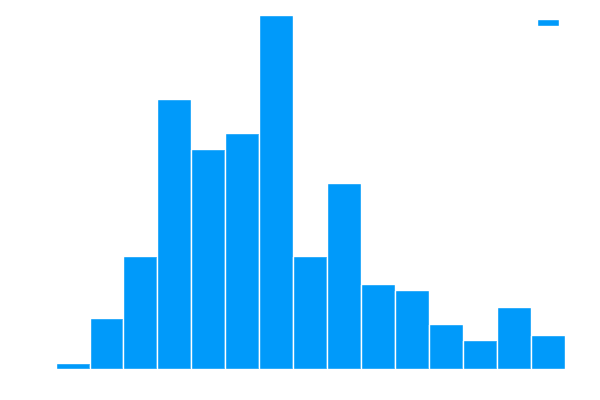
This method addresses the flawed sampling in bagging. Instead of sampling with uniform probability (which oversamples redundant data), the Sequential Bootstrap updates the sampling probabilities at each draw.

1. Draw 1: Sample $i$ with uniform probability $\delta_{i}^{(1)} = 1/I$.
2. Draw 2: Re-calculate the uniqueness of all labels given that sample $i$ was drawn. The probability of drawing sample $j$ for the second draw, $\delta_{j}^{(2)}$, is now proportional to its new average uniqueness $\bar{u}_{j}^{(2)}$.
   $$\delta_{j}^{(2)}=\bar{u}_{j}^{(2)}\left(\sum_{k=1}^{I} \bar{u}_{k}^{(2)}\right)^{-1}$$

This process makes it less likely to draw samples that heavily overlap with those already in the bag, resulting in a bootstrapped set that is closer to IID.

Solution 2: Sample Weights

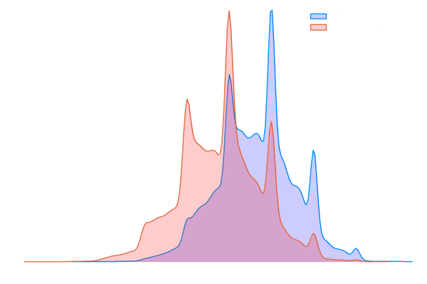
This section provides methods for weighting observations during model training, giving more importance to "better" samples.

Return Attribution

Weights are assigned based on both uniqueness and absolute return. The idea is to give more weight to unique labels that were associated with a significant market move. The weight $w_i$ is the absolute sum of all returns during the label's life, with each return $r_{t-1,t}$ divided by its concurrency $c_t$.

• Un-normalized weight:
  $$\tilde{w}_{i}=\left| \sum_{t=t_{i, 0}}^{t_{i, 1}} \frac {r_{t-1, t}}{c_{t}} \right|$$
• Normalized weight (to sum to $I$):
  $$w_{i}=\tilde{w}_{i} \cdot I \cdot \left(\sum_{j=1}^{I} \tilde{w}_{j}\right)^{-1}$$

Time Decay

To account for adaptive markets, older data should be less relevant. A time-decay factor $d$ is applied to the sample weights.

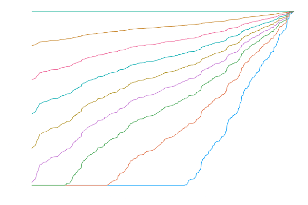
• Key Concept: The decay is not based on calendar time, but on cumulative uniqueness $\left( \sum \bar{u}_{i} \right)$. This prevents the model from rapidly discarding many recent, but redundant, observations.
• A parameter $c$ controls the decay rate, where $c=1$ is no decay, and $c < 0$ "forgets" the oldest portion of the data.

Class Weights

Finally, the text distinguishes sample weights (for uniqueness) from class weights.

• Class Weights: These are used to address imbalanced classes, not label overlap. If a model is trained to detect rare events (like a flash crash), class weights are applied to increase the penalty for misclassifying the rare event, forcing the model to pay more attention to it. A common setting for this is class_weight='balanced'.

Implementation: Uniqueness and Other Sample Weights

In our RiskLabAI.data.weights.sample_weights module, we implement the core functions for calculating sample weights to address the non-IID nature of financial data.

Concurrency and Uniqueness

We provide functions to measure the uniqueness of each label based on event concurrency.

1. Concurrency: First, we compute the number of concurrent events active at each timestamp. This function expands the event start/end times into a time series of active event counts.
2. Average Uniqueness: Using the concurrency data, we calculate the average uniqueness of each label, $\bar{u}_{i}$, as the average of $1/c_t$ over the label's lifespan. This index_matrix is an indicator matrix (T x N) representing active events, which can be derived from expand_label_for_meta_labeling.

Return-Based Sample Weights

We also implement the return attribution method to weight samples based on their associated market impact. The weight is calculated as the sum of absolute log-returns during the event, normalized by the concurrency at each step.

Time-Decay Weights

Finally, we provide a function to apply a time-decay factor to any set of weights. This allows us to give more importance to recent observations, with the clf_last_weight parameter controlling how much the oldest observations are discounted (linearly).

API reference

RiskLabAI implements these in Python and Julia (signatures auto-generated from the package source):

def expand_label_for_meta_labeling(
    close_index: pd.Index,
    timestamp: pd.Series,
    molecule: pd.Index,
) -> pd.Series:

function expand_label_for_meta_labeling(
    close_index::AbstractVector,
    event_start::AbstractVector,
    event_end::AbstractVector,
    molecule::AbstractVector,
)

def calculate_average_uniqueness(
    index_matrix: pd.DataFrame,
) -> pd.Series:

function calculate_average_uniqueness(index_matrix::AbstractMatrix{<:Real})

def sample_weight_absolute_return_meta_labeling(
    timestamp: pd.Series, price: pd.Series, molecule: pd.Index
) -> pd.Series:

function sample_weight_absolute_return_meta_labeling(
    event_start::AbstractVector,
    event_end::AbstractVector,
    price_index::AbstractVector,
    price::AbstractVector,
    molecule::AbstractVector,
)

def calculate_time_decay(weight: pd.Series, clf_last_weight: float = 1.0) -> pd.Series:

function calculate_time_decay(weight::AbstractVector{<:Real}; clf_last_weight::Real = 1.0)

Full source: Python · Julia