Backtesting on Synthetic Data

This chapter argues that standard backtesting (historical simulation) is a flawed method for calibrating trading rules (like stop-losses and profit-taking barriers). This practice leads to backtest overfitting, where the rules are tuned to a single, random historical path and fail out-of-sample.

The solution proposed is to backtest on synthetic data. This method avoids overfitting by optimizing the trading rules based on the underlying stochastic properties of the asset, not on a single historical scenario.

The Problem: Backtest Overfitting of Trading Rules

A trading rule $R$ is defined by its stop-loss ($\underline{\pi}$) and profit-taking ($\bar{\pi}$) thresholds: $R:=\{\underline{\pi}, \bar{\pi}\}$.

The standard (and flawed) approach is to brute-force a historical backtest to find the rule $R^*$ that maximizes the in-sample Sharpe Ratio ($SR_R$):

This $R^*$ is overfit because it targets specific in-sample outliers and is not fit for the future.

The Solution: An Optimal Trading Rule (OTR) from Synthetic Data

The chapter proposes a method to find the Optimal Trading Rule (OTR) by modeling the price series as a stochastic process.

1. Model the Stochastic Process

The price is modeled as a mean-reverting Ornstein-Uhlenbeck (O-U) process, which is characterized by its mean-reversion speed ($\varphi$), volatility ($\sigma$), and long-term equilibrium price ($\mathrm{E}_{0}\left(P_{i, T_{i}}\right)$).

• O-U Process Equation:
  $$P_{i, t}=(1-\varphi) \mathrm{E}_{0}\left(P_{i, T_{i}}\right)+\varphi P_{i, t-1}+\sigma \varepsilon_{i, t}$$
• Half-Life: The mean-reversion speed $\varphi$ can be expressed by its half-life $\tau$:
  $$\tau=-\frac{\log [2]}{\log [\varphi]}$$

2. The Numerical Algorithm

Instead of a historical backtest, the OTR is found through a 5-step simulation:

1. Estimate Parameters: Use OLS on the entire historical dataset to estimate the O-U parameters $\hat{\varphi}$ and $\hat{\sigma}$.
   $$\hat{\varphi}=\frac{\operatorname{cov}[Y, X]}{\operatorname{cov}[X, X]} \quad \text{and} \quad \hat{\sigma}=\sqrt{\operatorname{cov}\left(\hat{\xi}_{t}, \hat{\xi}_{t}\right)}$$
2. Create a Mesh: Define a grid of all possible trading rules (e.g., 20 stop-loss values $\times$ 20 profit-take values).
3. Generate Synthetic Paths: Using the estimated $\hat{\varphi}$ and $\hat{\sigma}$, simulate a large number (e.g., 100,000) of new, synthetic price paths.
4. Evaluate Mesh: Test every rule from the mesh (Step 2) against all 100,000 synthetic paths (Step 3).
5. Find the OTR: Calculate the average Sharpe Ratio for each rule across all synthetic paths. The OTR is the rule $(\underline{\pi}, \bar{\pi})$ with the highest average Sharpe Ratio.

Key Findings & Conclusion

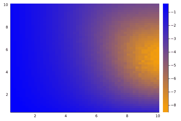
This method generates a "heat map" of Sharpe Ratios for all possible trading rules.

• The experiments show that when a genuine mean-reverting property exists (low $\tau$, positive forecast), a clear, stable optimal rule emerges.
• As the process approaches a random walk (high $\tau$), the heat map becomes noisy, and no stable optimal rule appears.
• This is the method's greatest strength: It prevents overfitting by confirming when no optimal rule exists, saving the researcher from "discovering" a false, overfit rule from a single historical path.

Advanced Synthetic Data: Markov-Switching Heston-Merton Model

While the Ornstein-Uhlenbeck process is useful for modeling mean-reversion, financial markets exhibit more complex behaviors, such as jumps and switching volatility regimes. In our RiskLabAI.data.synthetic_data.synthetic_controlled_environment module, we implement a powerful synthetic price generator that combines two models:

1. Heston-Merton Model: This model generates prices with stochastic volatility (Heston) and sudden price jumps (Merton).
2. Markov-Switching: The parameters of the Heston-Merton model (like drift, volatility-of-volatility, and jump intensity) are not constant. They are controlled by a hidden Markov-switching process, allowing the simulation to move between distinct regimes (e.g., "Bull Market," "Bear Market," "Crash").

Methodology

The core of the simulation is a Numba-optimized function that computes the log returns based on the Heston-Merton stochastic differential equations for price and volatility:

• Heston Volatility Process:
  $$v_{i+1} = v_i + \kappa_i (\theta_i - \max(v_i, 0)) dt + \xi_i \sqrt{\max(v_i, 0)} dwV_i \sqrt{dt}$$
• Merton Jump-Diffusion (Price):
  $$\log(S_{i+1}/S_i) = \left(\mu_i - 0.5 v_i - \lambda_i (m_i + \frac{v^2_i}{2})\right) dt + \sqrt{v_i} dwS_i \sqrt{dt} + dJ_i$$

API reference

RiskLabAI implements these in Python and Julia (signatures auto-generated from the package source):

def form_block_matrix(
    n_blocks: int, block_size: int, block_correlation: float
) -> np.ndarray:

function form_block_matrix(n_blocks::Integer, block_size::Integer, block_correlation::Real)

def drift_volatility_burst(
    bubble_length: int,
    a_before: float,
    a_after: float,
    b_before: float,
    b_after: float,
    alpha: float,
    beta: float,
    explosion_filter_width: float = 0.1,
) -> tuple[np.ndarray, np.ndarray]:

function drift_volatility_burst(
    bubble_length::Integer,
    a_before::Real,
    a_after::Real,
    b_before::Real,
    b_after::Real,
    alpha::Real,
    beta::Real;
    explosion_filter_width::Real = 0.1,
)

def compute_log_returns(
    n_steps: int,
    mu_vector: np.ndarray,
    kappa_vector: np.ndarray,
    theta_vector: np.ndarray,
    xi_vector: np.ndarray,
    dw_stock: np.ndarray,
    dw_vol: np.ndarray,
    jump_comp: np.ndarray,
    poisson_var: np.ndarray,
    dt: float,
    sqrt_dt: float,
    lambda_vector: np.ndarray,
    m_vector: np.ndarray,
    v_vector: np.ndarray,
    regime_change: np.ndarray,
) -> np.ndarray:

function compute_log_returns(
    n_steps::Integer,
    mu::AbstractVector,
    kappa::AbstractVector,
    theta::AbstractVector,
    xi::AbstractVector,
    dw_stock::AbstractVector,
    dw_vol::AbstractVector,
    jump_comp::AbstractVector,
    poisson_var::AbstractVector,
    dt::Real,
    sqrt_dt::Real,
    lambda::AbstractVector,
    m::AbstractVector,
    v::AbstractVector,
    regime_change::AbstractVector{Bool},
)

def align_params_length(
    regime_params: RegimeParams,
) -> tuple[dict[str, list[float]], int]:

function align_params_length(regime_params::AbstractDict)

def random_cov(num_columns: int, num_factors: int) -> np.ndarray:

function random_cov(num_columns::Integer, num_factors::Integer; rng = default_rng())

def form_true_matrix(
    n_blocks: int, block_size: int, block_correlation: float
) -> tuple[np.ndarray, np.ndarray]:

function form_true_matrix(
    n_blocks::Integer,
    block_size::Integer,
    block_correlation::Real;
    rng = default_rng(),
)

def simulates_cov_mu(
    mu0: np.ndarray, cov0: np.ndarray, n_obs: int, shrink: bool = False
) -> tuple[np.ndarray, np.ndarray]:

function simulates_cov_mu(
    mu::AbstractVecOrMat{<:Real},
    covariance::AbstractMatrix{<:Real},
    n_observations::Integer;
    shrink::Bool = false,
    rng = default_rng(),
)

def heston_merton_log_returns(
    total_time: float,
    n_steps: int,
    mu_vector: np.ndarray,
    kappa_vector: np.ndarray,
    theta_vector: np.ndarray,
    xi_vector: np.ndarray,
    rho_vector: np.ndarray,
    lambda_vector: np.ndarray,
    m_vector: np.ndarray,
    v_vector: np.ndarray,
    regime_change: np.ndarray,
    random_state: Optional[int] = None,
) -> np.ndarray:

function heston_merton_log_returns(
    total_time::Real,
    n_steps::Integer,
    mu::AbstractVector,
    kappa::AbstractVector,
    theta::AbstractVector,
    xi::AbstractVector,
    rho::AbstractVector,
    lambda::AbstractVector,
    m::AbstractVector,
    v::AbstractVector,
    regime_change::AbstractVector{Bool};
    random_state = nothing,
)

def generate_prices_from_regimes(
    regimes: dict[str, RegimeParams],
    transition_matrix: np.ndarray,
    total_time: float,
    n_steps: int,
    random_state: Optional[int] = None,
) -> tuple[pd.Series, np.ndarray]:

function generate_prices_from_regimes(
    regimes::AbstractDict,
    transition_matrix::AbstractMatrix{<:Real},
    total_time::Real,
    n_steps::Integer;
    random_state = nothing,
)

def parallel_generate_prices(
    number_of_paths: int,
    regimes: dict[str, RegimeParams],
    transition_matrix: np.ndarray,
    total_time: float,
    n_steps: int,
    random_state: Optional[int] = None,
    n_jobs: int = 1,
) -> tuple[pd.DataFrame, pd.DataFrame]:

function parallel_generate_prices(
    number_of_paths::Integer,
    regimes::AbstractDict,
    transition_matrix::AbstractMatrix{<:Real},
    total_time::Real,
    n_steps::Integer;
    random_state = nothing,
)

Full source: Python · Julia