Adapting to Regime Change

A model can respond to change in several ways: infer a latent state, raise an alarm when recent errors shift, or refit on a fixed schedule. The notebooks compare these choices without letting later outcomes alter earlier predictions.

The central relation

After observing return $r_t$ , a two-state filter updates its probability by

\pi_{t\mid t,j} =\frac{f_j(r_t)\pi_{t\mid t-1,j}} {\sum_{\ell=0}^{1}f_\ell(r_t)\pi_{t\mid t-1,\ell}}.

$j$ labels a state, $\pi_{t\mid t-1,j}$ is its probability before seeing the current return, and $f_j(r_t)$ is the fitted density of that return in state $j$ . The denominator makes the updated probabilities sum to one.

When market change calls for a model refit

The state plot follows the filtered probability through public returns. The policy comparison reports the recent prediction loss under static, scheduled, and alarm-driven refits.

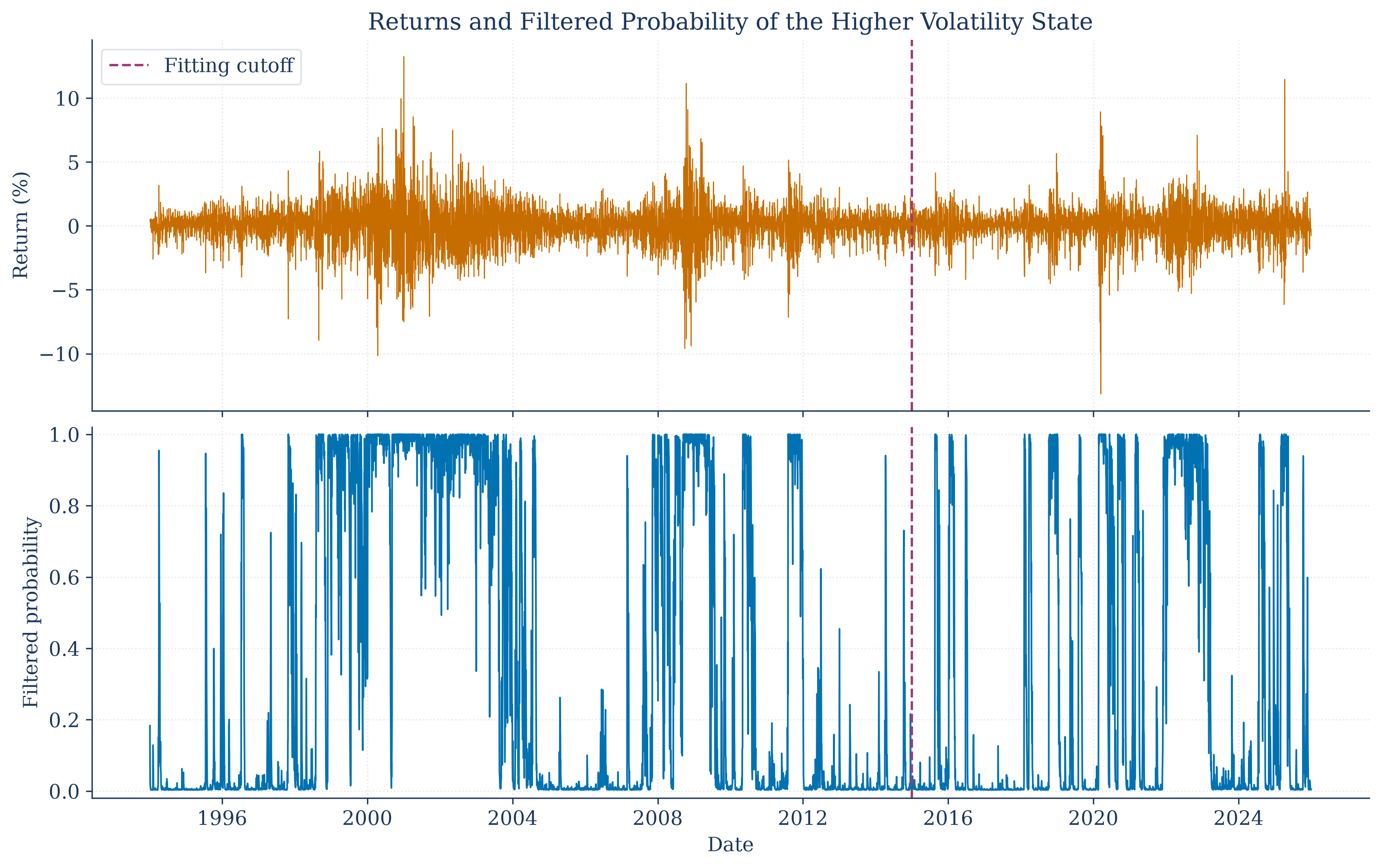
Filtered probability of a high-volatility state through public market observations. — The probability changes as each new return arrives while the fitted state parameters remain fixed during the evaluation period.

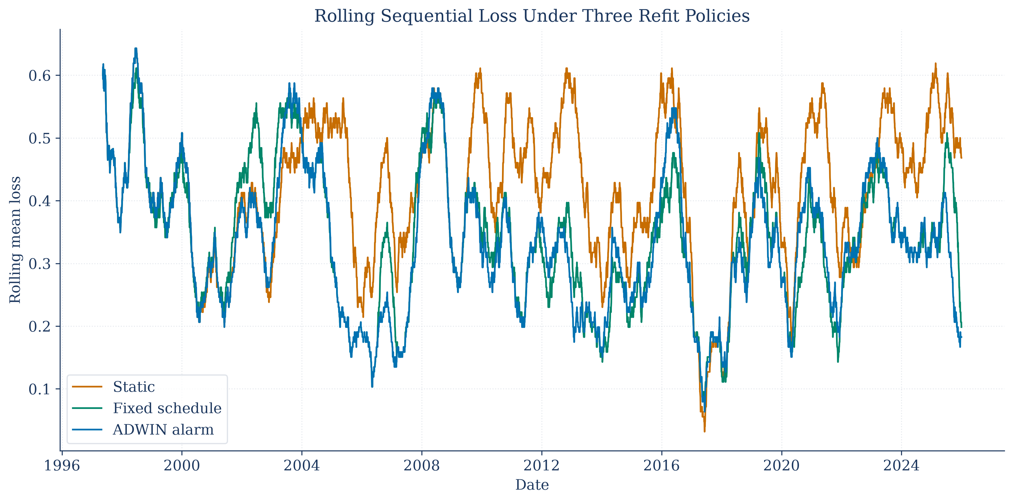
Rolling prediction loss for static, periodic, and alarm-driven model refit policies. — The rolling comparison uses the same features and outcome for all policies. Only the timing of model refits changes.

A fitted state is a statistical description, not a permanent economic regime. An alarm marks evidence of change under its stated rule; it does not identify the cause.

Notebooks


1. Inferring hidden regimes from filtered probabilities
2. Three Ways to Mark Change
3. Updating a Model After Change