Measuring Ambiguity in Probability Laws

Risk describes variation under one stated probability law. Ambiguity describes disagreement among several plausible laws. The notebooks keep those ideas separate and show how the answer changes with the supplied weights and probability grid.

The central relation

For mean bin probability $\bar p_k$ and across-law variance $v_k$ , the finite ambiguity measure is

A=\sum_{k=1}^{K}\bar p_k v_k, \qquad \bar p_k=\sum_{j=1}^{J}q_jp_{j,k}, \qquad v_k=\sum_{j=1}^{J}q_j(p_{j,k}-\bar p_k)^2.

$K$ is the number of outcome bins and $J$ is the number of supplied laws. Law $j$ receives weight $q_j$ and assigns probability $p_{j,k}$ to bin $k$ . The value $v_k$ measures disagreement about that bin, while $A$ combines the bin contributions.

Separating ordinary risk from ambiguity

The controlled example distinguishes ordinary risk from ambiguity. The public-data example then compares annual risk with disagreement among fitted monthly laws.

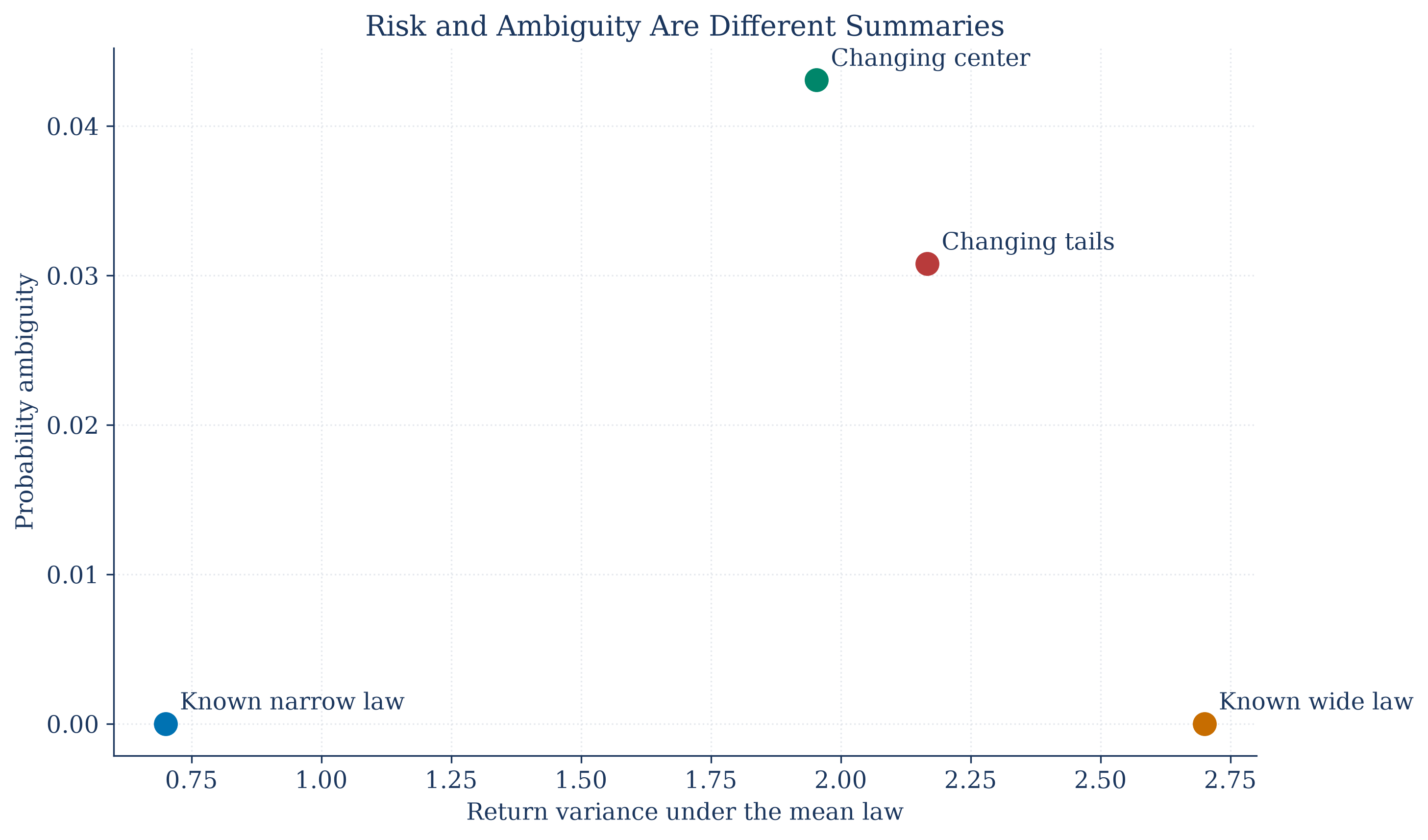
Controlled examples showing changes in risk and ambiguity across supplied probability laws. — The controlled cases show that dispersion within a law and disagreement across laws can move separately.

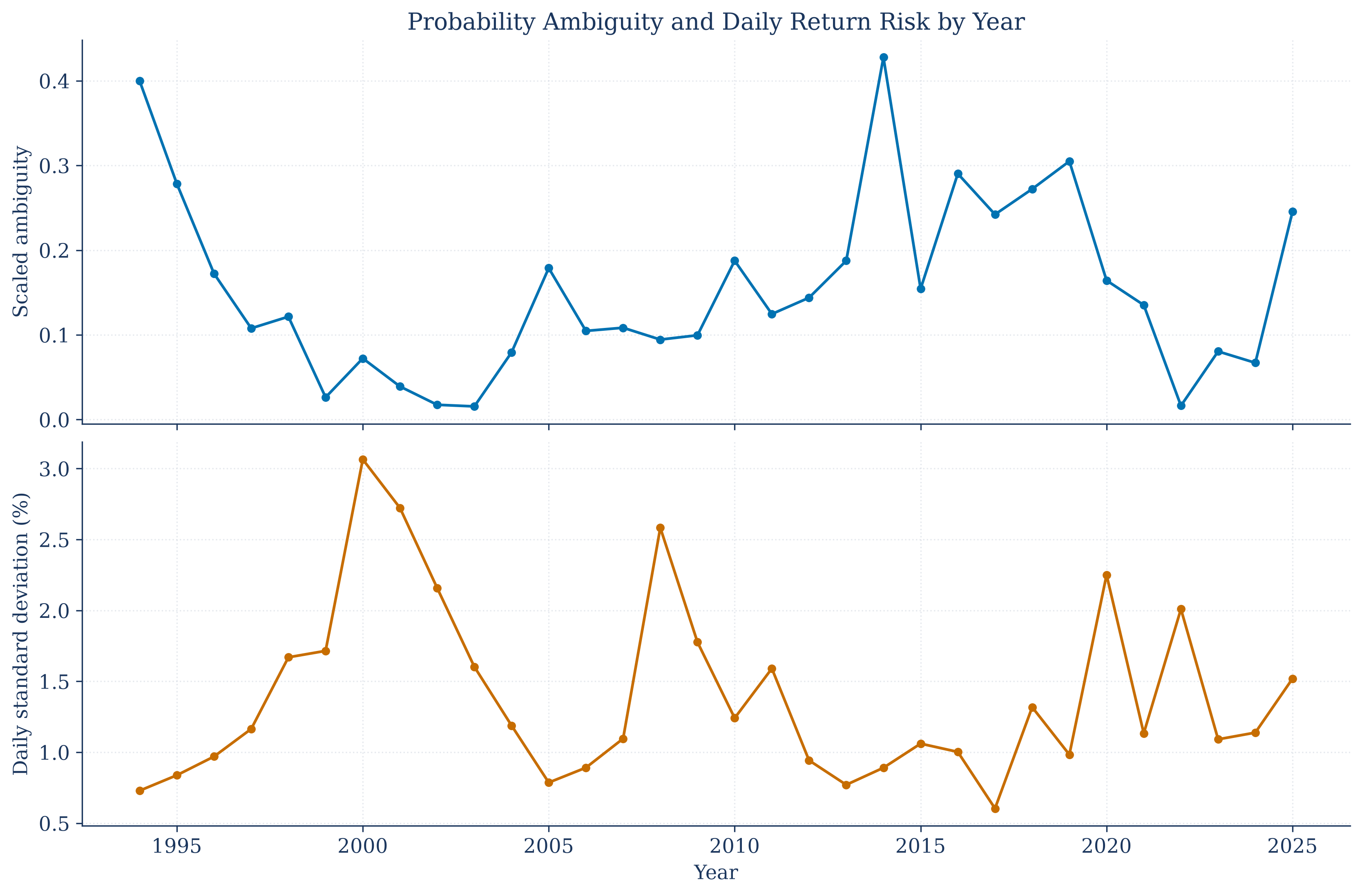
Annual ambiguity and return risk calculated from public NASDAQ Composite observations. — The public example compares realized return variation with disagreement among twelve fitted monthly laws. The two series answer different questions and need not move together.

The public calculation treats fitted monthly laws as a teaching construction, not as observed investor beliefs. Grid and weight checks remain part of the reported result.

Notebooks


1. Separating ambiguity from ordinary risk
2. A Finite Calculation from Supplied Priors
3. Measuring ambiguity in public market data